
The GEMS Informatics Grid Goes Open Source
We are delighted to announce that we have just released the GEMS Grid code library, where the code is under the open source Apache 2.0 license, which allows anyone to use the code for commercial or non-commercial purposes – you simply need to provide attribution to GEMS Informatics when you use or modify it.
Just before we at GEMS Informatics started developing Application Programmer Interfaces (APIs) in agriculture for GEMS Exchange, GEMS geospatial expert Jeffery Thompson worked with others in the GEMS team and colleagues at NSIDC to develop the GEMS Grid, a hierarchical discrete global gridding system. This Grid has allowed us to provide data sets at different resolutions ranging from 36 km to 1 m, and still have them remain functionally interoperable. The interoperability is possible because we have written the code to allow users to project data onto the grid, aggregate data to coarser resolutions, and, notably, also disaggregate data to finer resolutions. The latter operation is ordinarily a difficult problem, but is made easier, as I discuss below, since we enable the users of our code to thoughtfully address it in a standardized, replicable way.
Many problems in agriculture (e.g., understanding the spatial location of crop production) require equal area parcels of land to do proper calculations. Working with strict lat-lon coordinates won’t suffice as areas near the equator are significantly different in size as areas near the poles. The GEMS Grid preserves equal-area assumptions as it divides land, so you can do these calculations with confidence, and preserve aggregation-disaggregation consistency in the data, even if you are not a GIS expert.
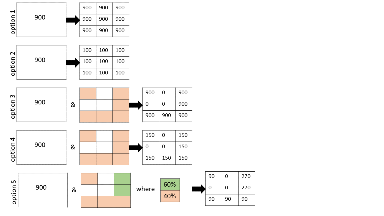
So let’s look at the 5 options for disaggregation that GEMS geospatial developer Olena Boiko included in the GEMS grid toolbox, schematically described in the figure she developed above.
Option 1. Value transference.
In this case, if you were to subdivide a 3 km2 resolution grid cell into 9 x 1 km2 cells, this option would be appropriate for any value that is deemed roughly constant throughout the area applied. Examples would be rainfall in inches or grain yield in bushels / acre.
Option 2. Even value division.
Sometimes the quantity measured in a cell represents a cumulative value for the area in which it is reported. In this case, if the parent cell is homogenous, then splitting it up into 9 equal-area pieces would require that you divide the value in each equivalent cell by a factor of 9. Examples where this selection makes sense include grain production in bushels, crop acreage, and population.
Option 3. Value transference with a mask.
This one is similar to Option 1 except we are no longer making the assumption that the distribution of values in the parent cell is spatially homogeneous. For example suppose you were measuring grain yield, but you knew that 3 of your nine cells had buildings occupying them (see white areas in the Figure). In this case you only transfer your values to 6 remaining cells (colored peach) that have arable land. Cells are binary with this option (i.e., either allowed a value or not).
Option 4. Even value division with a mask.
Analogously, you can mask out cells in the value division case when you know that your daughters cells are not all equal. This is just like the case in Option 3, except you divide your parent-cell value evenly by the number of viable daughter cells. In this pictorial example, there are 6 viable daughter cells, so each gets a value of 900/6 = 150. This would be appropriate if you were computing grain production in bushels and you had a total value that needed to be split up across the 6 arable daughter parcels.
Option 5. Flexible division with a mask.
This scenario is the most flexible, and allows the user to create a master mask with arbitrary weights at each daughter cell. It allows you to block off daughter cells entirely, and prescribe the relative weights of all remaining daughter cells. This is ideal for situations where you are allocating crop distributions and you want to avoid certain land use features (e.g., lakes, forests, housing) and probabilistically distribute the remaining crop areas (e.g., with higher probability near soils with a high SSURGO National Commodity Crop Productivity Index).
I’m confident these flexible disaggregation tools will provide much easier, more accurate, and replicable solutions for your particular spatial analytic problem. So please give them a try!
This activity supported in part by MnDRIVE Global Food Ventures, University of Minnesota